Throughput vs Latency: Optimizing Transformer Design for LLM Inference
 Sep, 14 2026
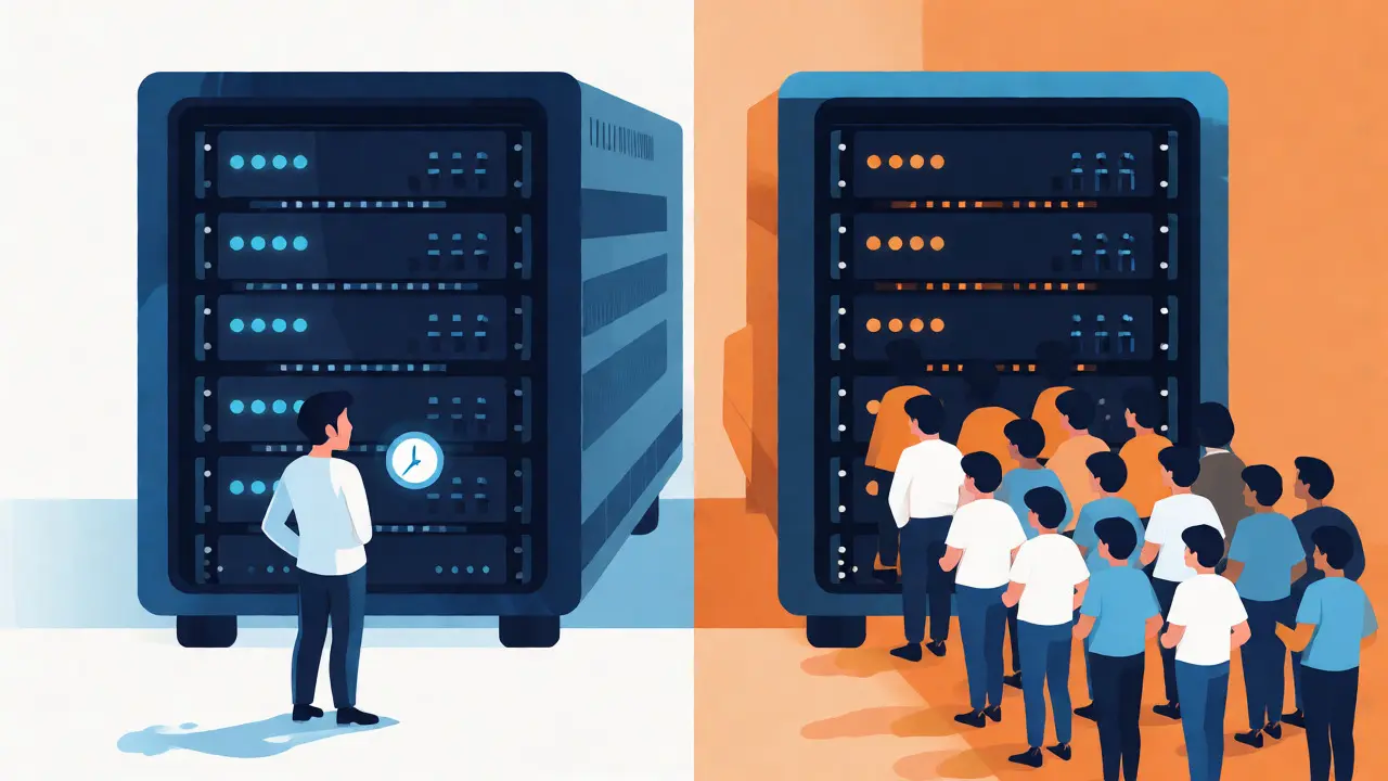
You’re building a chatbot. It works great in testing, but the moment you deploy it to production with real users, everything slows down. Or maybe you’re running a batch job to summarize thousands of documents, and your GPU bill is skyrocketing while the process crawls. What’s happening? You’ve likely hit the fundamental wall of Large Language Model (LLM) serving: the trade-off between throughput and latency.
These two metrics are constantly fighting each other. If you want to serve more users at once (high throughput), individual responses usually get slower (higher latency). If you want instant answers (low latency), you waste expensive GPU cycles on idle capacity (low throughput). There is no free lunch here. But understanding how Transformer architecture a deep learning model structure that relies on self-attention mechanisms to process sequences of data interacts with hardware can help you pick the right battle to fight.
Defining the Metrics That Matter
Before we talk about optimization, let’s clear up what these terms actually mean in the context of LLMs. They aren’t just buzzwords; they dictate your user experience and your cloud bill.
Latency the time delay between the cause and its effect in a system, specifically the time it takes for an LLM to generate a response isn’t a single number. It’s broken down into two critical parts:
- Time To First Token (TTFT): The wait time from when a user hits "send" until the first word appears. This is where the model processes the entire prompt (prefill phase).
- Time Per Output Token (TPOT): How long it takes to generate each subsequent word after the first one.
Total latency is TTFT plus (TPOT × total output tokens). If you have a short answer, TTFT dominates. If you have a long essay, TPOT matters more.
Throughput the rate at which a system processes requests, measured in tokens per second across all concurrent users measures efficiency. It tells you how many tokens your server can spit out per second if you throw enough work at it. High throughput means you’re squeezing every drop of performance out of your NVIDIA A100 or H100 GPUs.
| Metric | Primary Driver | User Impact | Cost Impact |
|---|---|---|---|
| TTFT | Prompt length & Batch size | Perceived responsiveness | Low impact on cost |
| TPOT | Model size & Memory bandwidth | Reading speed comfort | Moderate impact |
| Throughput | Batch size & Hardware utilization | Scalability limits | High impact (efficiency) |
The Batching Dilemma
Here is the core mechanic causing the friction: Batching processing multiple inference requests simultaneously to maximize GPU utilization. GPUs love big batches. They are designed to perform matrix multiplications on large blocks of data. When you send one request at a time, the GPU spends most of its time waiting for data to move around rather than doing math. This is called being "memory-bound."
When you increase the batch size, you amortize the cost of fetching model weights from memory across multiple requests. Suddenly, the GPU is busy computing. Throughput skyrockets. Research shows that on a single A100 GPU, moving from a small batch to a batch size of 64 can increase throughput by 14x. Sounds great, right?
But there’s a catch. Larger batches mean new requests might have to wait in line behind existing ones. This inflates TTFT. If your batch is full, a new user’s prompt sits idle until a slot opens up. For interactive apps like chatbots, this feels sluggish. For background tasks like summarization, it’s perfectly fine.
The behavior also differs between the two phases of inference:
- Prefill Phase: Processing the input prompt. This is compute-heavy. Even a single request can saturate the GPU’s compute units. Batching helps less here because the GPU is already busy.
- Decode Phase: Generating output tokens one by one. This is memory-bandwidth heavy. Each token requires reading the entire model weights again. Here, batching is magic. It allows you to share that expensive weight-fetching cost among many users.

Scheduling Strategies: Who Goes First?
How your server decides which requests to process together determines your performance profile. Modern systems use different scheduling policies to balance the load.
Request-Level Batching a strategy where the system waits for a group of requests to arrive before processing them as a single unit is simple but inefficient. It stalls new requests until the current batch finishes decoding. This creates high latency spikes for new users but keeps implementation simple.
Iteration-Level Batching a dynamic scheduling method that adds new requests to the active batch at each generation step, popularized by frameworks like vLLM, is smarter. It lets new requests join the party immediately. As soon as a user finishes generating their last token, a new user jumps in. This dramatically improves throughput-often by an order of magnitude compared to older methods-because the GPU never idles waiting for a whole batch to finish.
However, even iteration-level batching has a trade-off. Prefilling a new long prompt can stall the decoding of ongoing requests. To fix this, newer schedulers like Sarathi-Serve interleave prefill and decode operations. By breaking long prefills into smaller chunks, they prevent any single request from hogging the GPU, smoothing out latency spikes while maintaining high throughput. This approach has shown improvements of up to 6.9x in throughput for large models like Falcon-180B while staying within strict latency limits.
Tensor Parallelism: Speed vs. Cost
What if your model is too big for one GPU? You split it across multiple GPUs using Tensor Parallelism (TP) a technique that partitions model layers across multiple devices to distribute memory and computation.
TP reduces latency because each GPU handles a smaller slice of the calculation. However, it introduces a hidden tax: communication overhead. When layers are split, GPUs must talk to each other frequently to combine partial results. This happens twice per transformer layer: once after attention and once after the feed-forward network.
Crucially, the amount of data sent between GPUs doesn’t shrink as you add more GPUs. The computation per GPU goes down, but the communication stays roughly constant. This increases the communication-to-compute ratio. Eventually, adding more GPUs yields diminishing returns. Your latency might drop slightly, but your throughput per GPU plummets. You end up paying for four GPUs to do the work of two-and-a-half. Always measure the actual benefit before scaling TP aggressively.

Choosing Your Optimization Target
So, should you optimize for throughput or latency? It depends entirely on your application.
If you are building a real-time chat interface or a code editor assistant, prioritize low TTFT. Users hate staring at a blinking cursor. Accept lower throughput and higher costs per token to keep the interaction snappy. Quadrant II of the performance graph (low TTFT, low throughput) is your sweet spot.
If you are running batch jobs-like translating millions of sentences or analyzing customer support tickets-optimize for throughput. No one cares if the first word takes 5 seconds to appear if the whole job finishes faster and cheaper. Maximize batch sizes and ignore minor latency spikes. Quadrant I (high TTFT, high throughput) might be acceptable if you have massive parallelism.
For mixed workloads, aim for a balanced point on the Pareto frontier. Use tools that allow dynamic batch sizing. Monitor not just average latency, but the 99th percentile. An average response time of 200ms looks good, but if 1% of users wait 5 seconds, they will churn.
Practical Tips for Better Performance
You don’t need to rewrite the transformer architecture to see gains. Start with these engineering adjustments:
- Monitor Goodput: Don’t just count tokens. Count tokens that meet your Service Level Objective (SLO). If a response arrives late, it’s worthless to the user. Goodput measures useful output per second.
- Optimize Prompt Length: Long prompts kill TTFT. If possible, truncate context or use retrieval-augmented generation (RAG) to keep inputs concise.
- Use Quantization: Running models in FP16 or INT8 reduces memory bandwidth requirements, directly improving TPOT without changing the transformer design.
- Profile Communication: If using multi-GPU setups, check if NVLink bandwidth is saturated. Sometimes switching from Tensor Parallelism to Pipeline Parallelism helps if communication is the bottleneck.
Is high throughput always better for business?
Not necessarily. High throughput lowers the cost per token, which is great for margins. But if it causes high latency, users may abandon the service. For interactive applications, poor user retention often outweighs infrastructure savings. Balance both based on user expectations.
Why does my Time To First Token (TTFT) spike under load?
This usually happens due to head-of-line blocking in the scheduler. If a long prompt is being processed (prefilled), new requests may wait for the current batch to complete. Using iteration-level batching or chunked prefill techniques can mitigate this by allowing new requests to interleave with ongoing generation.
Does increasing batch size always improve performance?
No. While larger batches improve GPU utilization and throughput, they eventually hit a ceiling where the system becomes compute-bound. Beyond this point, increasing batch size only increases latency without boosting throughput. Additionally, very large batches can exhaust High Bandwidth Memory (HBM), causing crashes or swapping.
How does tensor parallelism affect latency?
Tensor parallelism generally reduces latency by splitting computational work across multiple GPUs. However, it introduces communication overhead between GPUs. If the interconnect bandwidth (like NVLink) is slow, the communication time can negate the computational speedup, leading to worse overall performance.
What is the difference between prefill and decode phases?
The prefill phase processes the entire input prompt in parallel, making it compute-intensive. The decode phase generates output tokens sequentially, one by one, making it memory-bandwidth intensive. Batching helps significantly in the decode phase but offers limited benefits in the prefill phase for single requests.