Transformer Layers in Production LLMs: Memory and Compute Footprints
 Jun, 22 2026
Deploying large language models (LLMs) in production is less about the magic of AI and more about a brutal game of Tetris with silicon. You have massive models like Llama 3 or GPT-4, and you need them to run fast and cheap. But there is a wall standing in your way: the memory and compute footprints of transformer layers are the fundamental building blocks of modern neural networks that process data through attention mechanisms. If you don't understand how these layers eat up GPU memory and processing power, your deployment will either crash from out-of-memory errors or bleed money on cloud bills.
The core problem isn't just that models are big. It's that they behave differently depending on what you ask them to do. Sometimes the bottleneck is moving data (memory-bound), and sometimes it's doing math (compute-bound). Mixing these up leads to wasted resources. This guide breaks down exactly where your resources go, why the Key-Value (KV) cache is your new enemy, and how to optimize for real-world performance without sacrificing accuracy.
The Anatomy of Transformer Layer Costs
To fix the cost issue, you first need to know where the weight sits. A transformer layer consists primarily of two components: the Multi-Head Attention mechanism and the Feed-Forward Network (FFN). In production, these create two distinct types of resource consumption: static memory for weights and dynamic memory for activations.
Let's look at the numbers. Take Meta's Llama 2 7B, a popular open-source model. If you load this model in standard 16-bit precision (FP16 or BF16), the model weights alone take up roughly 14 GB of VRAM. That calculation is simple: 7 billion parameters multiplied by 2 bytes per parameter. However, this is only the entry fee. The real complexity comes from the dynamic elements during inference.
| Component | Size Estimate | Dependency |
|---|---|---|
| Model Weights | ~14 GB | Fixed (Parameter Count × Precision) |
| KV Cache (4K Context) | ~2 GB | Linear (Sequence Length × Batch Size) |
| Activations (Prefill) | Variable | Quadratic (without FlashAttention) |
The table above shows that while weights are static, the Key-Value (KV) cache scales with context length. For a sequence of 4,096 tokens, the KV cache adds another ~2 GB. But if you double the context to 8,192 tokens, that cache doubles too. This linear growth is manageable until you hit long-context applications like legal document analysis or codebase indexing, where the cache can explode.
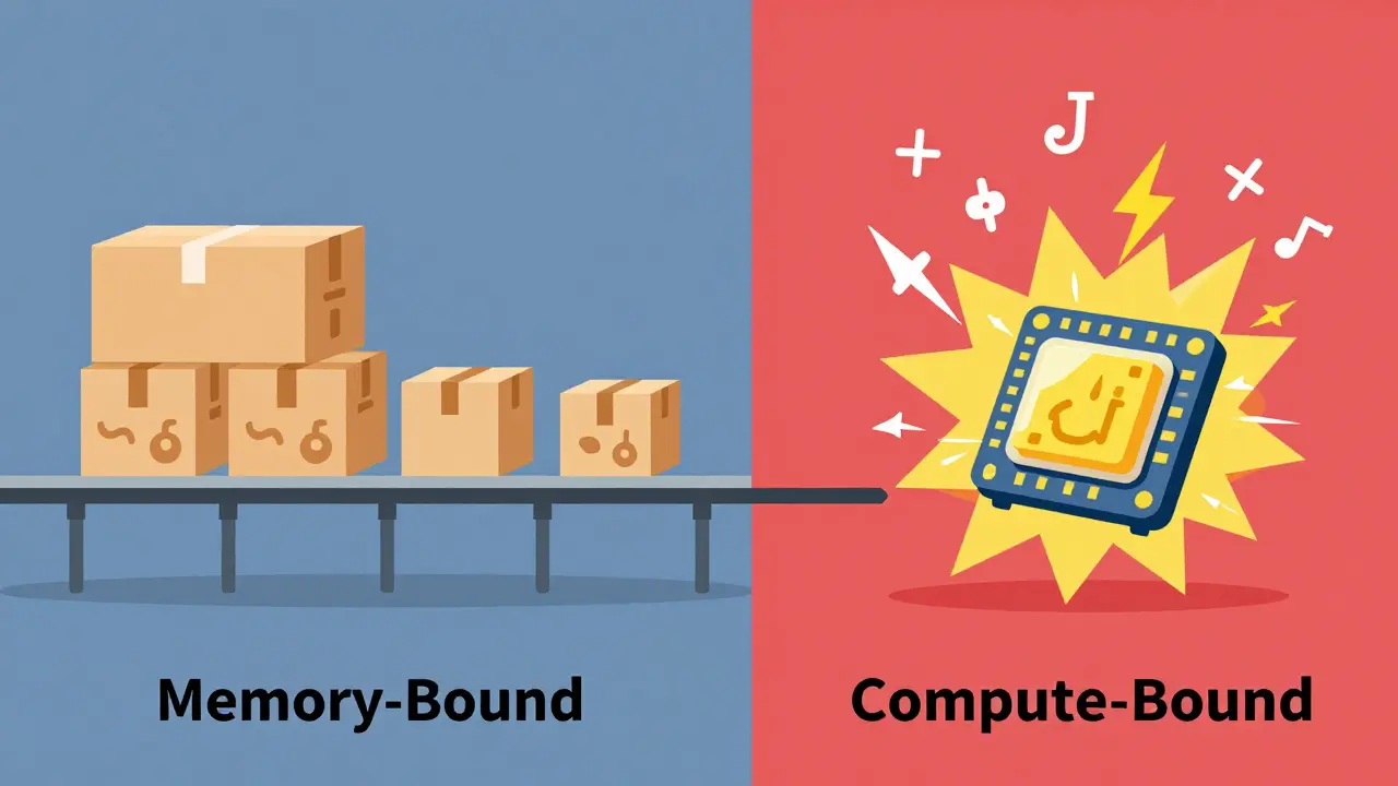
Memory-Bound vs. Compute-Bound Operations
This is the most critical distinction for any ML engineer deploying LLMs. Your optimization strategy depends entirely on which phase dominates your workload. Misidentifying this leads to "optimizing" the wrong thing, resulting in zero throughput gains.
Memory-Bound Phases: These occur when the GPU is waiting for data to arrive from memory rather than performing calculations. Loading model weights and accessing the KV cache are classic examples. In small-batch inference (e.g., one user chatting at a time), the GPU often sits idle because the memory bandwidth is saturated moving the heavy weights into registers. Here, reducing memory footprint via quantization helps significantly.
Compute-Bound Phases: These happen when the GPU is fully utilized doing math. The prefill stage (processing the initial prompt) is heavily compute-bound because it involves calculating attention scores for all tokens simultaneously. Research from Snowflake in September 2024 showed that for enterprise workloads using Llama 3.1, prefill computation dominates latency. In these cases, compressing the KV cache does little good; you need faster matrix multiplication or better kernel fusion.
A common mistake is applying aggressive KV cache compression to a compute-bound workload. As Snowflake’s data indicated, compressing the cache by 30× yielded less than 3% throughput improvement because the bottleneck was the arithmetic logic units (ALUs), not the memory bus. Conversely, trying to speed up memory-bound tasks by adding more GPUs without addressing data movement overhead results in diminishing returns due to communication latency.
The KV Cache Bottleneck
If there is one entity causing more headaches in production LLM deployments today, it is the Key-Value (KV) Cache. During autoregressive generation, the model must remember previous tokens to predict the next one. Instead of recalculating attention for every prior token, it stores keys and values in a cache.
The formula for KV cache size is straightforward but punishing:
M_KV = 2 × L × H_KV × d_head × bytes_per_cache × Sequence_Length
Where:
- L is the number of layers (e.g., 32 for 7B models).
- H_KV is the number of key-value heads (often reduced via Grouped-Query Attention).
- d_head is the head dimension (typically 128).
- bytes_per_cache is the precision (2 for FP16, 1 for INT8).
Dr. Younes Belkada, CEO of vLLM, noted in August 2024 that for sequences longer than 8K tokens, the KV cache memory consumption exceeds the model weights themselves in 70B+ parameter models. This shifts the bottleneck from storing the brain (weights) to storing the short-term memory (activations).
For example, running a 70B model with a 32K context window on an NVIDIA A100 cluster requires meticulous management. One Reddit user reported spending 45 minutes optimizing just to fit the KV cache, losing 22% throughput to pipeline parallelism overhead. The solution isn't just bigger GPUs; it's smarter caching strategies like PagedAttention (used in vLLM), which manages memory non-contiguously to reduce fragmentation.
Optimization Techniques That Actually Work
Knowing the bottlenecks allows you to apply targeted fixes. Here are the most effective techniques for reducing footprints in 2026.
1. Quantization
Quantization reduces the precision of model weights and activations. Moving from FP16 (16-bit) to INT8 (8-bit) cuts memory usage by 50%. Prem AI’s January 2024 report confirmed this reduction, showing significant cost savings for enterprise workloads. However, be cautious with INT4. Dr. Anna Rohrbach of Berkeley AI Research warned that aggressive quantization below INT8 risks quality degradation, showing an 8.7% accuracy drop on the MMLU benchmark for 70B models. Use INT8 for general chat and reasoning tasks; reserve INT4 for edge devices where latency is paramount and slight hallucination tolerance exists.
2. FlashAttention
Standard attention has quadratic complexity O(n²) relative to sequence length, meaning doubling the context quadruples the memory and compute required. FlashAttention is an algorithmic optimization that reduces memory usage from quadratic to linear by tiling computations. Dao et al.’s implementation achieved a 2.33× speedup on A100 GPUs. FlashAttention-2 further reduced scratch memory, enabling 128K sequence lengths on 80GB GPUs compared to the 4K limit of naive implementations. If you are running long-context tasks, FlashAttention is non-negotiable.
3. Parallelism Strategies
When a single GPU can’t hold the model, you split it. Choose wisely:
- Tensor Parallelism: Splits individual layers across GPUs. Best for compute-bound workloads. Low communication overhead but requires high-bandwidth NVLink connections.
- Pipeline Parallelism: Splits different layers across GPUs. Better for memory-bound scenarios where each GPU holds a chunk of the model. However, it introduces "bubble" time where some GPUs wait for others, costing 15-20% efficiency according to NVIDIA benchmarks.
Hardware and Future Architectures
Software optimizations have limits. The hardware landscape is evolving to address the von Neumann bottleneck-the delay caused by shuttling data between memory and processor. Compute-in-Memory (CIM) architectures are emerging technologies that perform calculations directly within memory cells to eliminate data transfer delays. A June 2024 arXiv survey documented 3.7× energy efficiency improvements and 5.2× speedups on transformer workloads using CIM prototypes from IBM and Samsung. While commercial CIM chips remain experimental, they represent the future of efficient inference.
Current production hardware like the NVIDIA Blackwell B200 (announced March 2024) addresses immediate needs with 192GB of HBM3e memory, specifically designed to accommodate massive KV caches. Meanwhile, startups like Groq and Cerebras offer alternative architectures focused on deterministic, low-latency inference by removing memory hierarchy constraints entirely.
Practical Deployment Checklist
Before pushing your LLM to production, run through this checklist to avoid costly failures:
- Profile First: Use tools like NVIDIA Nsight Systems to determine if your workload is memory-bound or compute-bound. Don't guess.
- Select Precision: Default to INT8 for models >13B parameters. Validate accuracy on your specific dataset before switching to INT4.
- Enable FlashAttention: Ensure your inference engine (vLLM, TensorRT-LLM) uses FlashAttention-2 or higher for any context window >4K tokens.
- Manage KV Cache: Implement PagedAttention or similar virtual memory techniques to prevent fragmentation in long-session applications.
- Choose Parallelism: Use Tensor Parallelism for high-throughput batch jobs; use Pipeline Parallelism if you are constrained by per-GPU memory capacity.
The market for LLM inference optimization grew to $2.8B in Q2 2024, reflecting the urgency of these issues. With 83% of Fortune 500 companies now deploying optimized LLMs, the competitive advantage lies not in having the biggest model, but in running it most efficiently. By mastering the memory and compute footprints of transformer layers, you transform AI from a cost center into a scalable product feature.
What is the difference between memory-bound and compute-bound inference?
Memory-bound inference occurs when the GPU spends more time waiting for data (weights/KV cache) to move from memory than performing calculations. This is common in small-batch serving. Compute-bound inference happens when the GPU is fully utilized doing math, typical during the prefill stage of long prompts. Identifying which dominates your workload dictates whether you should prioritize quantization (for memory) or kernel optimization (for compute).
How much memory does the KV cache consume?
The KV cache grows linearly with sequence length and batch size. For a 7B model in FP16, a 4K context window consumes approximately 2 GB. However, for larger models like 70B with 32K contexts, the KV cache can exceed the size of the model weights themselves, becoming the primary memory bottleneck.
Is INT4 quantization safe for production?
INT4 quantization reduces memory by 75% but carries risks. Research indicates an 8.7% accuracy drop on complex reasoning benchmarks (MMLU) for 70B models. It is suitable for edge devices or applications tolerant of minor hallucinations, but INT8 is generally recommended for enterprise-grade reliability unless rigorous calibration is performed.
Why is FlashAttention important for long contexts?
Standard attention algorithms require memory proportional to the square of the sequence length (O(n²)). FlashAttention reduces this to linear complexity (O(n)) by using tiling and IO-aware algorithms. This enables handling context windows of 128K+ tokens on consumer-grade GPUs that would otherwise run out of memory at 4K tokens.
Should I use Tensor or Pipeline Parallelism?
Use Tensor Parallelism if your workload is compute-bound and you have GPUs connected via high-speed NVLink, as it minimizes communication overhead. Use Pipeline Parallelism if you are memory-bound and need to split a large model across GPUs with limited interconnect bandwidth, accepting a 15-20% efficiency loss due to pipeline bubbles.